We used a CO2 isotherm apparatus to measure the pressure P and volume V of a CO2 sample at various temperatures T for a fixed amount n of gas. We used the Van der Waals equation:
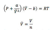
where R is the gas constant, T is the temperature, a and b are parameters to be investigated. V bar is the molar volume and n is the number of moles in the volume. Long-range intermolecular potential is a and the short range intermolecular potential is given by b. At high T or low density, the equation behaves like the ideal gas law, PV = nRT. Therefore, the volume of the CO2 sample depends both on the temperature, pressure, and the number of moles present. We will investigate this relationship.
The apparatus we used was really old, and hadn’t been cleaned since 1999. Therefore, we expected our measurements to have large uncertainties. The apparatus consisted of a capillary tube containing a fixed amount of CO2, which was compressed with an oil-mercury pump. The pump compressed the oil, which then moved the mercury and in turn compressed the CO2. Since the pump controlled the compression of the CO2 sample, it also controlled the pressure the CO2 was subject to. We were able to measure this pressure with a pressure gauge.
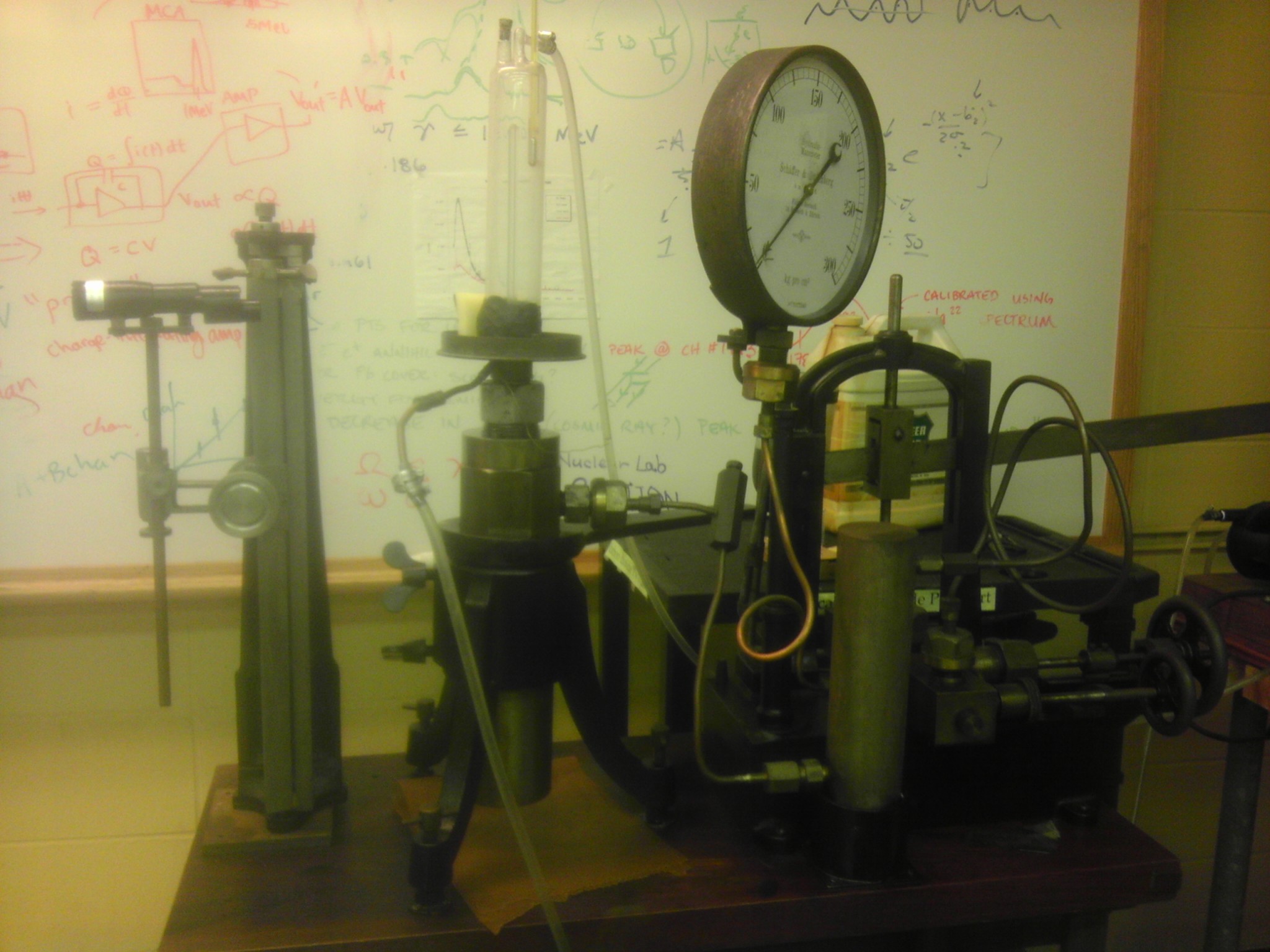
The apparatus. We measured the height of the mercury with the telescope on the left. The pressure gauge is to the right and the CO_2 sample is in the glass tube.
We measured the temperature with a mercury thermometer placed beside the capillary tube. We wanted to change the temperature of the CO2 sample and keep it constant. Therefore we pumped water with a certain temperature into the outer tube that contained the capillary tube, which was called a cooling jacket. The water came from a large vat, where we could heat it with three A.C. electric heaters supplied by a variable voltage source. But since this took forever, we just boiled water in an electric teapot and dumped it into the vat. We still had to wait for the temperature of the water in the cooling jacket to stabilize and equal the temperature of the water in the vat, but this would only take about five to ten minutes instead of three hours.
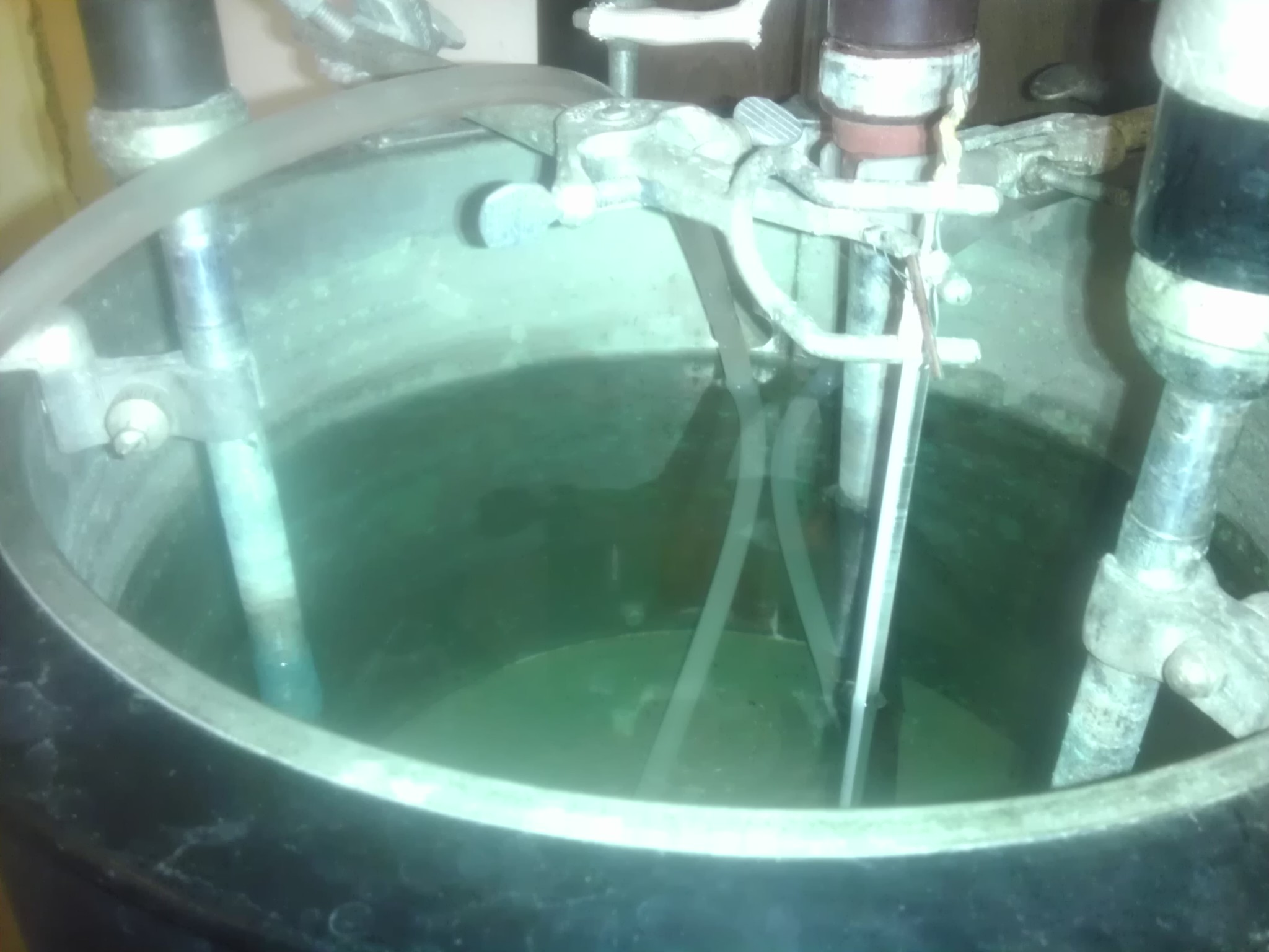
The vat of water and the three heaters. During the experiment we also had a thermometer so that we could compare the temperature of the water in the vat and in the capillary tube.
The temperature of the water had to be constant in order for us to reduce the uncertainty in our measurements, but this was difficult to achieve. The temperature of the water in the vat after some time would start decreasing because it was exposed to room temperature. Also, the cooling jacket leaked, especially when the temperature of the water was high. We stopped the leaking with play-dough and a sponge from the physics kitchen (we had to get a new sponge afterwards).
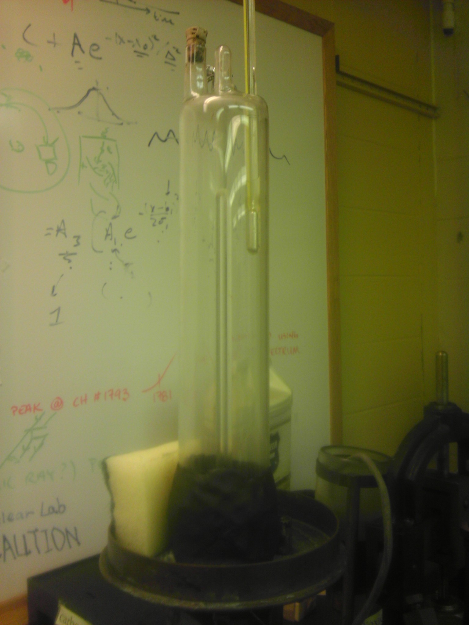
The cooling jacket, and the capillary tube. The thermometer was placed in the cooling jacket, near the capillary tube. Note the black play-dough and sponge on the base which helped us prevent or control leaks.
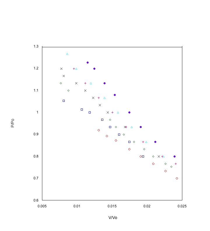
We first calibrated the apparatus by measuring the height of the capillary tube, which we found to be 40.5 cm. The height of CO2 was the difference between the height of the capillary tube and the mercury. We then took seven runs of data at seven different temperatures: 28.6°C, 33.3°C, 35.9°C, 39.0°C, 41.9°C, 44.2°C, and 50.2°C. We took data by varying the pressure inside the capillary tube and measuring the height of the mercury. Afterwards, we plotted the P/P0 vs V/V0. P0 and V0 are given constants for C02, where P0 = 7.38 × 10⁶ Pa and V0 = 94.0 cm3 mol-1. We came up with the following graph:
We knew that the behavior of real gases can be modeled with the following virial equation:
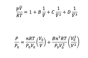
The first equation is the virial equation. The second equation, was derived from the virial equation and used to fit our data
B, C, and D are virial coefficients that become progressively smaller for higher order terms of V. We discarded all higher order terms because they were too small to affect the curve fit. We knew the value of all of the variables except for n and B. The n value is constant for all temperatures, but B is temperature dependent. In order to calculate for n and B, we fit the data to a curve and solved for n and B. We fit our data to the second equation shown above, which was derived from the first equation.
| T (K) | 301.6 | 306.3 | 308.9 | 311.9 | 314.9 | 317.2 | 323.2 |
| n (moles x 10-3) | 6.3 | 5.5 | 5.7 | 5.5 | 5.9 | 5.7 | 6.1 |
| B (cm3 mol-1) | -93 | -82 | -76 | -75 | -75 | -73 | -71 |
Some of the curve fits we found were not ideal because they would dip for low temperatures and didn’t fit the data very well at those points. This was probably due to the fact that the curve fit we used had that “shape.”
We then took all of the n values, averaged them and found it was 5.8×10⁻³ moles. We recalculated all the B values using this value and found:
| T (K) | 301.6 | 306.3 | 308.9 | 311.9 | 314.9 | 317.2 | 323.2 |
| B (cm3 mol-1) | -93 | -82 | -76 | -75 | -75 | -73 | -71 |
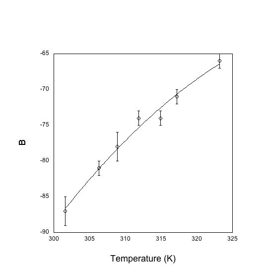
| B recalculated | -87±2 | -81±1 | -78±2 | -74±1 | -74±1 | -71±1 | -66±1 |
We graphed the recalculated values for B vs Temperature (K), and although the B values were bigger than expected the curve fit was a second order polynomial as expected. Give the age and condition of our apparatus, the larger B values could be explained as a result of the uncertainty of our measurements.
Although we did not find the Van der Waals parameters a and b, we did find the B values for each temperature. This lab was really fun and exciting, even though it yielded measurements with giant uncertainties.

