In this experiment I calculated the electric charge of an oil drop by measuring the force it experienced from a known electric field. I also calculated how the force, on a charged particle, varied when the electric field changed. Since the force exerted by an electric field on an object with very little charge is also very small, I had to observe tiny oil drops falling and rising really small distances. The main result of this experiment was that focusing on tiny dots for more than 15 minutes made my vision blurry.

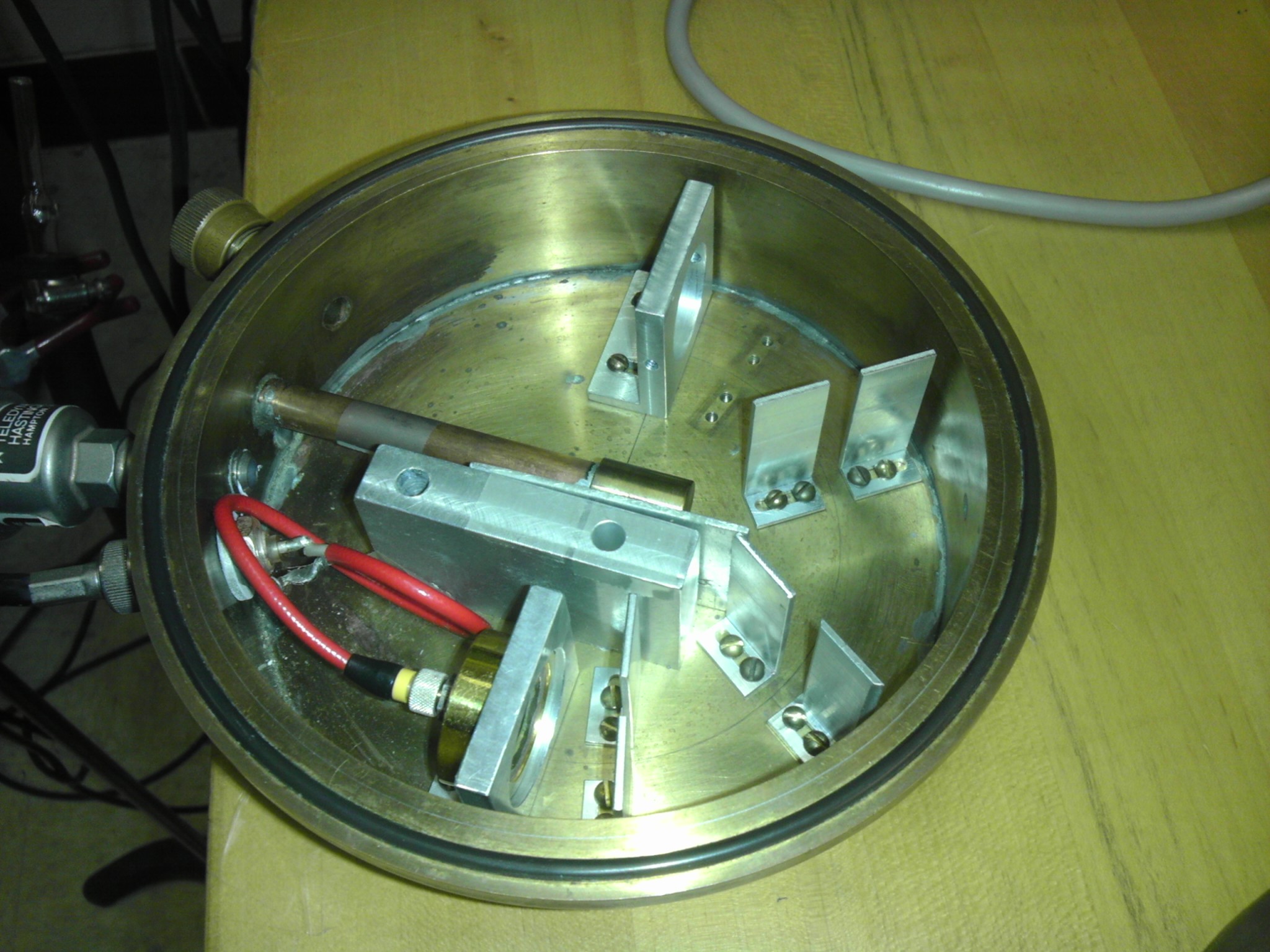
The experiment consisted of a two plate capacitator that had a plastic spacer between them. The capacitator was placed within a chamber and had a small hole in the middle where I could introduce the oil drops . There was also a viewing scope mounted so that I could see the hole in the spacer and observe the falling oil drops. I was able to see the drops thanks to a halogen lamp that illuminated the drops. The viewing scope had a grid, whose major lines were separated by 0.5 mm, that allowed me to measure the distance the drops fell.

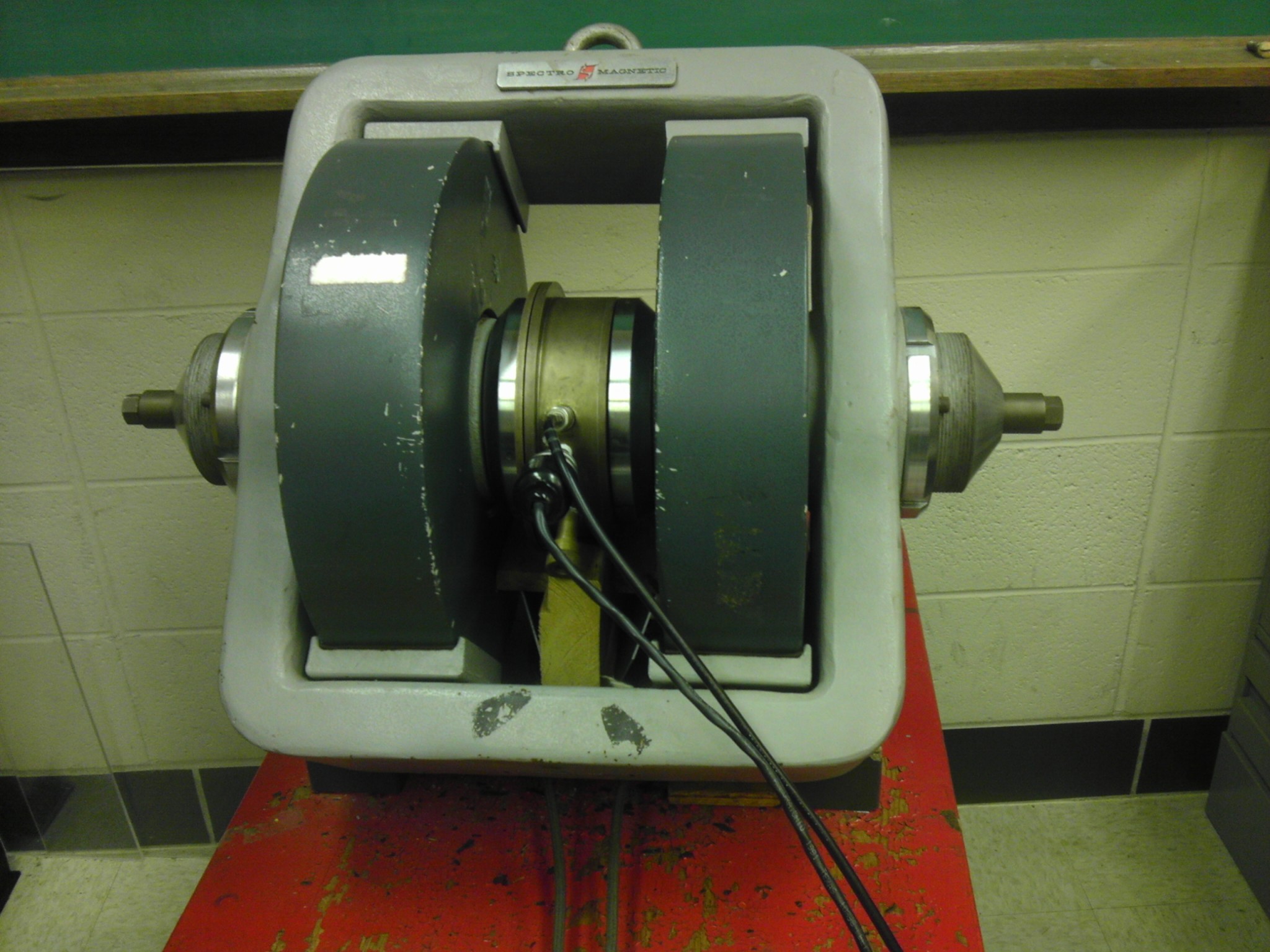
The oild drops I saw through the scope were kind of like this, just smaller and bright gold.

The capacitators were given voltage by a high voltage DC power supply. There was also a thermistor mounted on the bottom capacitator plate. A thermistor is a resistor whose resistance varies a lot with temperature, and I measured its resistance with a multimeter. With the given resistance I was able to calculate the temperature within the chamber, which was important for later calculations. Lastly, there was an ionization source within the chamber that could be turned on and off. This would create excess electrons that attached themselves to some of the oil drops, and increased their electric charge.

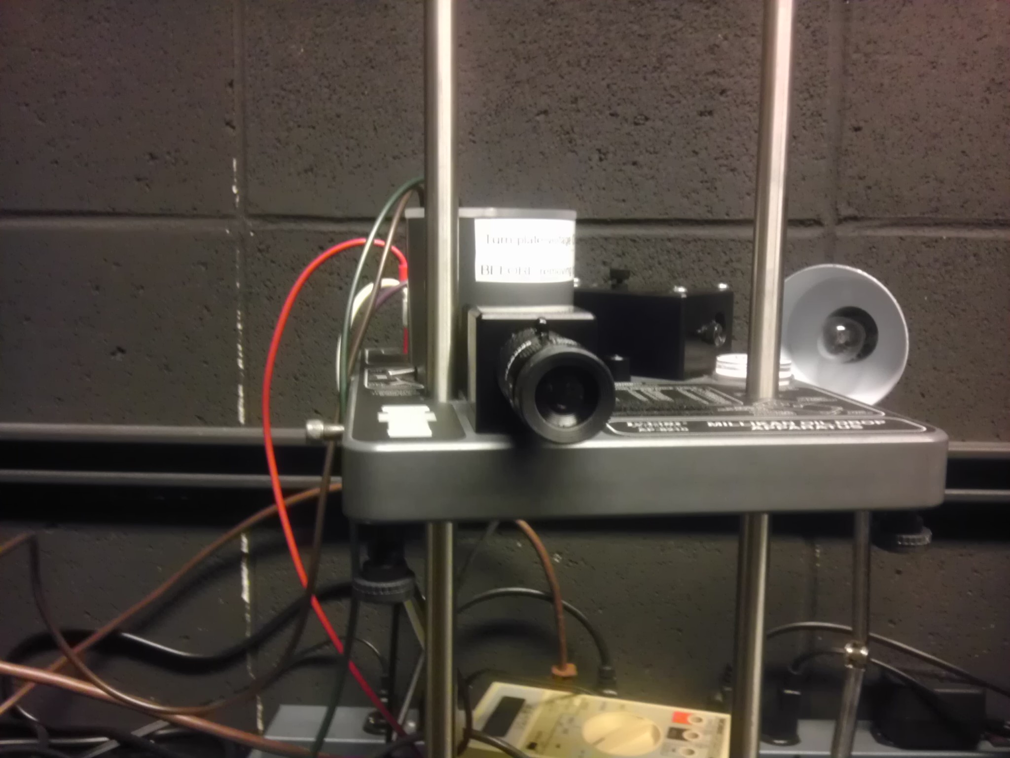
The viewing scope is right in front of the cylindrical chamber, and is placed at eye level.

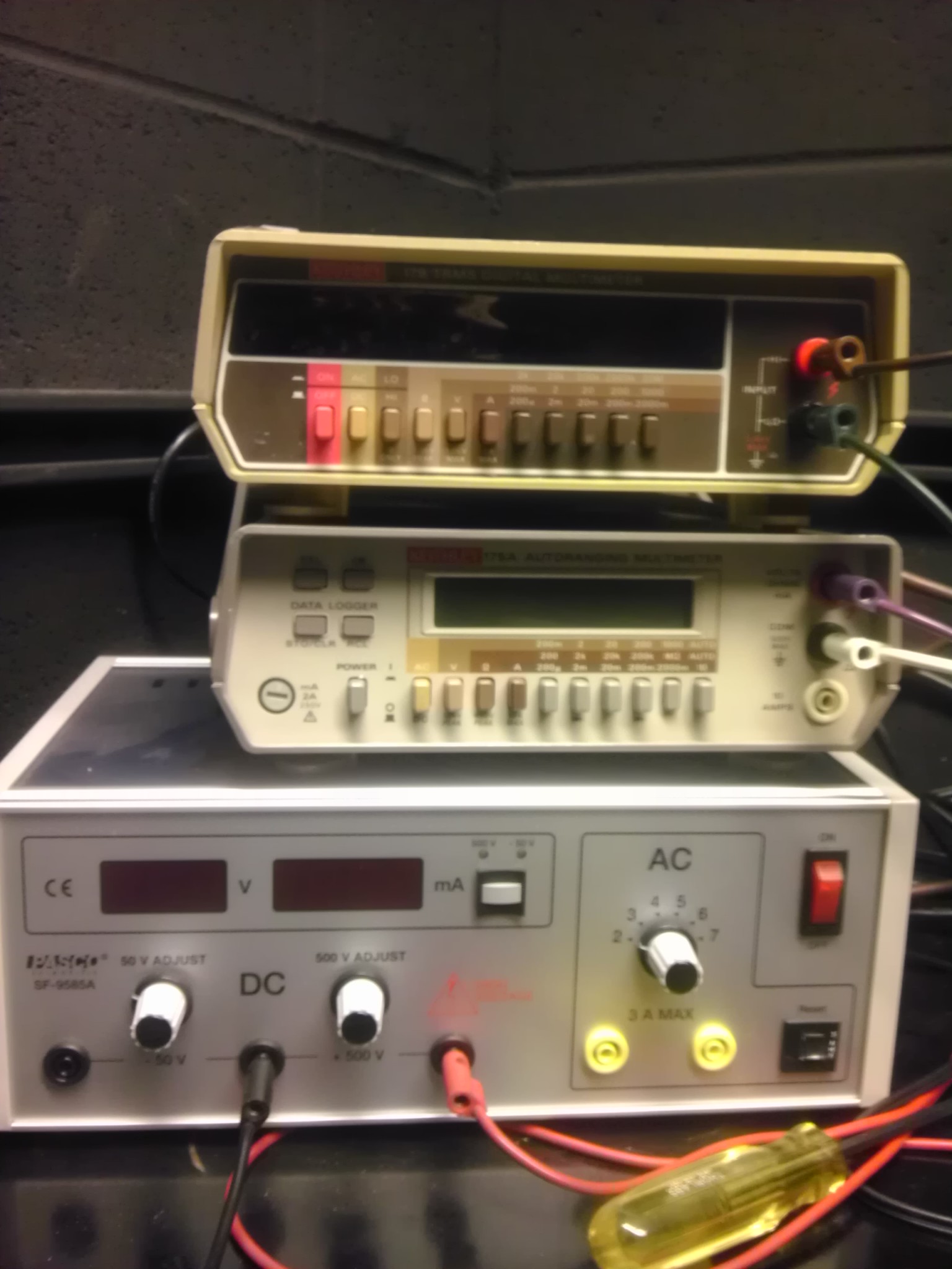
The high voltage DC power supply is on the bottom. Above it, there are two multimeters.

I observed the fall and rise of oil drops in the chamber because the force they experienced also affected their velocities. The force from the electric field would speed up the drops fall and rise. On the other hand, gravity slowed the rise of the particles, so the oil drops velocity was different if it was falling or rising. It seems a little crazy that oil drops can rise, but that was possible because I could reverse the polarization of the electric field. When I did this, I made the electric field and the force point upwards.

It took me forever, but I was able to choose a single oil drop and make it fall and rise in different electric fields, caused by different voltages. I measured the time it took to fall and rise a distance of 0.5 mm, with a voltage of 306.5v, 397v, 483v, 206.2v and 103.1v. I observed that the greater the voltage was, the smaller the time interval was.

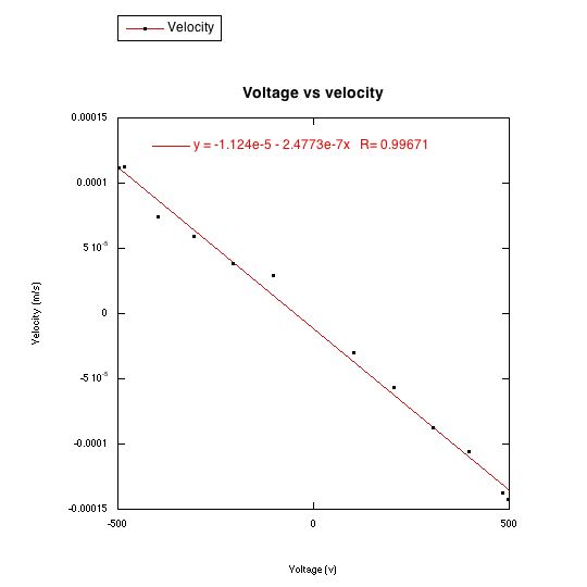
The velocity of falling and rising drops in different voltages increases linearly with voltage. Note that the graph is not centered at the origin.

I also measured the fall and rise of a drop that was exposed to the ionization source. I did not change the electric field and kept the voltage at 245.7 volts. First, I measured the velocity of the drop without turning on the ionization source. Then, I turned on the ionization source for 5 s, and measured the velocity of the drop. I turned on the source one last time and measure the velocity of the drop again. When I turned on the source, it emitted excess electrons that attached themselves to the drops. This increased the charge of the drop and as a result increased the force and the velocity of the drop. This occurred in the first time I turned on the source, but the second time the drop slowed down considerably. Something happened so that the drop didn’t gain electrons, but lost them.

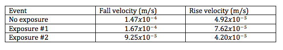
The drop was exposed to an ionization source for 5 second intervals. Curiously, the second exposure resulted in the drop losing electrons instead of gaining them.

I was able to calculate the electric charge of each drop whose velocity I measured, as well as the drop whose charge changed. I did this with the following equation:

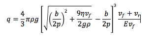
I found the charge of the electron with this equation

I calculated the charge of each drop, divided it with the charge of the electron and rounded up the result. The drop I whose velocity I measured as function of voltage had six electrons. The drop that wasn’t exposed to the source in the field created by a voltage of 2457 v had 14 electrons. The drop then gained 4 electrons, and had a charge of q=18 e. The drop was exposed a second time to the source and it lost 10 electrons, so it had a charge of q=8e. The loss of electrons cannot be explained as the result of the ionization source, but it is possible another drop stole the electrons. There might be another, better explanation.

In conclusion, the Millikan oil drop experiment is a very pretty experiment and the fact that you can measure the charge of the electron so precisely is kind of amazing. On the other hand, it was very difficult to NOT to lose a drop, and it took hours to find a drop that was a “perfect match” (Wenqi’s words). So, I’m not sure whether I like this experiment or not.

I measured the gamma decay of various sources, such as 22-Na, 66-Co, 137-Cs, and 133-Ba. I also measured the gamma decay of 5 brazil nuts, which were surprisingly radioactive. I used a hyper-pure germanium detector that was kept at a temperature of 77K with liquid nitrogen. The detector consisted of a semiconductor, characterized by a conduction band and a valence band. If an electric field is applied, the electrons in the valence band are stuck and can’t increase their conductivity. But if we apply a change in temperature, the electrons can jump to the conduction band. Another way that electrons are liberated is when they’re hit with a gamma ray and are given some of the gamma’s kinetic energy. The gamma ray then scatters with the remainder of it’s kinetic energy and will either escape or hit another electron, repeating the process until it runs out of kinetic energy or escapes.

The detector sweeps up the liberated electron with a high voltage, and sends a pulse to the preamplifier. The detector was kept at a very low energy because the high voltage might excite other electrons thermally and “cover up” the pulse created by the gamma rays. The preamplifier creates a voltage pulse whose height is proportional to the energy of the liberated electrons. The preamp’s pulse is sent to an MCA, were it’s amplified and shaped before being measured. The MCA creates a histogram of channel vs counts, were a spread of channels corresponds to a pulse height and as a result to the energy of the gamma ray.

I first measured the gamma decay of 66-Cobalt, and found two peaks. Each peaks corresponded to single gamma rays with a defined kinetic energy KE. As a result, the peaks are also called photopeaks. The photopeaks also tell us that the gamma rays were fully captured, so all of their KE was passed onto the electrons. Since I didn’t know how the channel number was related to the energy of the gamma’s, I looked up what the energy values should be for this source. They were 1.173 MeV and 1.332 MeV.

The peaks correspond to two fully captured gamma rays with different kinetic energies.

I also measured the gamma decay of 137-Cesium where the back scatter peak and the Compton edge were clearer than in 66-Co. When a gamma ray collides with an electron, it will “bounce” at an angle wrt its original trajectory. So if a gamma ray bounces back with a 180 degree angle, it is basically going back the way it came from. If the gamma ray manages to escape after a single collision, only a fraction of it’s KE is detected. The gamma ray can give the electron a maximum amount of KE, if it bounces back with a 180 degree angle. Therefore, on the spectrum we can see an edge that has a peak and falls off because the gamma has given the most KE it can without being absorbed. The backscattered peak occurs when the gamma scatters without being detected and then scatters again until it is fully absorbed. In fact the energy value of the backscattered peak equals the energy of the Compton edge subtracted from the energy value of the photopeak.

The Compton edge and the back scattered peak are well defined, and the photopeak corresponds to a fully captured gamma with a kinetic energy of 662 keV.

I also measured the gamma decay of Barium and sodium. I related the channel number to the KE value by looking up the KE of the photopeaks for each source. My data fit a line perfectly and I was able to identify the KE of any gamma decay measured by the detector I used.

I used the given KE values for each source in order to find the relationship between the channel number and KE value. Note that it’s a perfect fit.

I wanted to measure the gamma decay of brazil nuts and find out what radioactive isotopes formed it. I had to measure the background radiation first, so that when I measured the radiation of the brazil nuts I could tell which peaks were due to background radiation. Since the background radiation was so “weak” I had to leave the detector running for 24 hrs.

Note that there were at least three major photopeaks, and that there were few gamma rays present with a high KE value

I then measured the gamma radiation of brazil nuts for 24 hrs. The photopeaks that were present in the background spectrum also showed up, so I was able to weed them out. I found that the remaining photopeaks corresponded to Radium-224, Potasium-43 and Protactinium-234. Further analysis might show that brazil nuts contain other radioactive isotopes as well.

Observe that there are more photopeaks than in the background spectrum. These peaks corresponded to the radioactive isotopes within the brazil nuts

In this experiment I measured the maximum kinetic energy  of a source that emits beta particles and is experiencing a magnetic force.

Beta decay occurs when an atom has too many neutrons or protons and one decays into the other. This decay results in the emission of a neutrino and either a positron or electron. Beta decay was the first clue to the existence of the neutrino. The neutrino was needed to account for the loss of energy and momentum that was measured from the emitted particles.

I had a detector inside a brass chamber, where we could place the source perpendicularly to the detector or right in front of it. The detector measured the electrons emitted by the source  This chamber was connected to a Preamplifier, and to a Voltage supply so that we could create a current within the chamber.

The output pulse of the detector went though the preamp, an amplifier and an oscilloscope before going into the CANBERRA Series 35 Plus. The Canberra collected the data and created a histogram of channel number vs counts, where the channel number was proportional to the energy of the pulse.

Note how the source can be placed directly in front of the detector or 180 degrees away from it. Also note that we use slits to define the radius of curvature of the beta rays emitted by the source.

In order to determine the relationship between the channel numbers and the energy values, I measured the known maximum kinetic energies (KEmax) of the sources. I found a spectra for Srontium, Chlorine-36, Thalium-204 and Technetium-99 and measured the channel where KEmax occurred.

The thalium had a smaller maximum Kinetic Energy than the strontium and the chlorine, which was not what we had expected given their known maximum kinetic energies.

The known KEmax (763 keV) of Thalium is bigger than that of chlorine (708 keV) and strontium (546 keV). Since I measured it as smaller than the KEmax of chlorine and strontium I had to discard it for my calibration line.

I only used our data from the strotium, chlorine and techerium sources. I discarded the thalium source data because the measured KEmax was smaller than we expected.

I proceeded to measure the Energy of chlorine-36 in different magnetic fields. I placed the source 180 degrees away from the detector and evacuated the chamber. Then, I placed it between the two magnets. A current was fed into the magnets by the   which produced a magnetic field that was constant in the radial direction of the chamber. I measured the strength of the magnetic field within the chamber with a gaussmeter. I measured the source’s energy peak as a function of current. As I was doing this the CANBERRA died, and I lost two of my spectra.

I measured the energy peaks from the data I hadn’t lost and graphed it vs the magnetic field I had measured squared over the kinetic energy. I only used three data points since I lost the rest. On the other hand, the line is within error. The line had a slope of -68.487 and an intercept of 2.8512.

I plotted B^2/K vs K in order to calculate the charge of the electron and the rest energy of the electron E_0. Unfortunately my data did not fit a line well, and the uncertainty is of the fitted line is very high. This uncertainty is due to the uncertainty of the energy calibration and to the fact that there was very little data to work from.

The line I found corresponded to the following equation. As a result we can find the charge of the electron and the rest energy E_0.

This equation is derived in the lab write-up

 I calculated the electron charge to be e=1 x 10 ^(-8) C, which was not within error of the standard value, e=-1.6021765 x10^(-19) C. The rest energy, which depended on e, was equal to 3.311 x10^(-4) joules. From this we can find the electrons rest mass because E_0=m c^2, where m is the electrons rest mass. The rest mass is equal to 3.6788 x10^(11) kg which was still very different from the standard value 9.109×10^(-31) kg. The gigantic uncertainty of these values is due to various factors, firstly the energy calibrations uncertainty. It is also due to the uncertainty in measuring the peak of the data and determining K. Furthermore, I lost data and I cannot determine whether any of the three point can or cannot be discarded.